Reinforcement Learning 102: Q-learning & SARSA

Introduction

In the previous article, we derived Value Iteration. The update was:

This is a model-based update. It assumes that we know the environment dynamics:

If this distribution is available, the update can evaluate actions before choosing one. For each possible action $a$ in state $s$, it averages over all possible rewards $r$ and next states $s^\prime$ to compute that action’s candidate value. Once every action has been evaluated this way, the outer $\max_a$ selects the best one and uses it to update $v(s)$.

In most real problems, we do not know $p(r, s^\prime \mid s, a)$ in advance. One way forward is to learn this model from data and then plan with it. This is also close to how people often reason: before acting, we imagine what might happen next and whether it will be good or bad. For example, stealing something may lead to getting arrested.

But learning an explicit dynamics model is not trivial. Yann LeCun makes a related point in his work on predictive world models: useful prediction should often happen at a more abstract level than raw pixels. If the state is everything visible on the screen, then predicting the exact next state means predicting the next image pixel by pixel, including details that may not matter for the decision.

To learn in this model-free setup, we need samples from interaction with the environment. They may come from the current agent, another policy, or an existing dataset, but each sample still records what happened along one realized path. We cannot pause in state $s$, try every possible action, observe all possible outcomes, average them, and then go back to choose the best action. Some policy chooses one action, gets one reward, moves to one next state, and the episode continues.

So instead of the exact model-based update, interaction gives us samples from the unknown dynamics. A single transition looks like:

Over time, these sampled transitions form trajectories, episodes, or rollouts. This is the data source for the rest of the article. The next question is what we should estimate from those samples so that we can improve a policy.

Use Q, not V

One tempting idea is to use rollouts to estimate $v(s)$ like we did in previous article. That works for prediction, but it is not enough for control. The reason is simple: $v(s)$ tells us how good state $s$ is under some policy, but it does not tell us which action to choose in that state. In the model-based setting, this was not a problem. If we knew $v(s)$ and the transition model, we could compare actions by computing:

Then we could improve the policy greedily:

In the model-free setting, this path is blocked. We do not know $p(r, s^\prime \mid s, a)$, so we cannot turn $v(s)$ into action comparisons. Estimating $v(s)$ alone would tell us that a state is good or bad, but not which action made it good or bad. So for model-free control we should learn action-values directly:

The action-value function answers the question we need for control: if I am in state $s$ and take action $a$, what return should I expect? Once we have an estimate $q(s, a)$, we can extract a greedy policy without a transition model:

That is why the rest of the article focuses on learning $q(s, a)$ from sampled rollouts.

Estimation methods

Before looking at control algorithms, we first need two ways to estimate $q(s, a)$ from sampled experience.

Monte Carlo

Monte Carlo learning uses complete episodes. Suppose an episode produces the following trajectory:

The episode ends in terminal state $S_T$. After it finishes, we can compute the realized return from each time step:

For every visited state-action pair $(S_t, A_t)$, this $G_t$ is one sample of the return after taking action $A_t$ in state $S_t$. The estimate $q(s, a)$ does not depend on time; it is tied to the state-action pair. The time index is only needed to identify which sampled return $G_t$ came from the rollout.

To write the estimate without carrying the time index everywhere, let $s = S_t$ and $a = A_t$ for a sampled visit. Across episodes, or even within one episode, the same state-action pair may appear many times, and each visit gives another sampled return. Monte Carlo estimates the action-value by averaging those returns:

Here $N(s, a)$ is the number of observed returns for that state-action pair. We do not need to store all previous episodes to compute this average. When we observe a new return for $(s, a)$, we first increment the count:

Then we treat the new return as $G_i(s, a)$ and update the running average:

Equivalently:

The cost is that we must wait until the episode finishes. If the episode is very long, or if the task is continuing and does not naturally end, this can be inconvenient. Monte Carlo returns can also have high variance, because a full return may depend on many random events that happen after the current state-action pair. Averaging over more episodes reduces this variance, but it may take many samples.

Sparse rewards make this worse. A reward signal is sparse when most transitions produce zero or uninformative reward, and useful feedback appears only after a rare event. Imagine a game where the agent receives a meaningful reward only after winning. If the initial policy is random, the agent may play many episodes without ever winning, so most sampled returns contain no useful learning signal. In that case Monte Carlo learning may need a large number of samples before it observes even one successful trajectory.

Temporal Difference

Monte Carlo gives us a clean sampled target, but it has one practical problem: we need to wait for the final return.

Temporal Difference (TD) learning changes the target. Instead of waiting for the complete return $G_t$, it uses the recursive Bellman equation for action-values and bootstraps from the current estimate. This is the same Bellman expectation idea from the previous article, where we used it for $v_\pi$, but unrolled one step further so that the value is attached to a state-action pair. For a fixed policy $\pi$, the equation for $q_\pi$ is:

This says: take action $a$ in state $s$, receive reward $r$, move to $s^\prime$, and then follow policy $\pi$ from the next state. If we knew the transition distribution, we could compute that expectation exactly.

There are two expectations inside this equation. The outer one is over the environment dynamics $p(r, s^\prime \mid s, a)$. In a model-free setting, we do not know those probabilities, so this is the part we must replace with a sampled transition:

That sampled transition is enough to handle the unknown transition probabilities. It does not, by itself, require the transition to be generated by the same policy $\pi$ that appears in the Bellman equation. Once we condition on $(s, a)$, the reward and next state come from the environment dynamics $p(r, s^\prime \mid s, a)$. Which policy collected the sample matters for coverage and for the action distribution used in the target, and we will return to that in the on-policy vs. off-policy section.

The inner expectation is over the next action under the policy $\pi$. That part is different: if we know the policy and the current action-value estimates, we can either sample one next action from $\pi$ or compute the expectation over actions directly.

If we sample the next action $a^\prime \sim \pi(\cdot \mid s^\prime)$, the one-step sample is:

and its target is:

This version samples both the environment outcome and the next action under $\pi$. There is another possibility: keep the action expectation instead. Then the transition $(s, a, r, s^\prime)$ is enough, and the target becomes:

We will come back to that difference when we compare SARSA with Expected SARSA. For now, assume the sampled-action target $(s, a, r, s^\prime, a^\prime)$ and:

This target can be used immediately after observing $s^\prime$ and choosing $a^\prime$. It gives us more frequent updates than Monte Carlo, but it bootstraps from the current action-value estimate $q(s^\prime, a^\prime)$, which may still be wrong. It also has extra noise from sampling $a^\prime$.

The TD update has the same shape as the Monte Carlo running-average update:

For Monte Carlo, the target was the sampled return $G_i$, and the step size was often $\frac{1}{N(s, a)}$. For a sampled-action TD target, the target is the bootstrapped estimate $r + \gamma q(s^\prime, a^\prime)$. Because this target is noisy and also depends on the current value estimate, we usually use a learning rate $\alpha$ instead of $\frac{1}{N(s, a)}$:

The term in parentheses is the error between the bootstrapped target and the current estimate. Equivalently, the same update can be written as:

With a constant $\alpha$, this behaves like an exponential moving average: recent targets receive more weight, but older targets still influence the estimate indirectly through the previous value of $q(s, a)$.

We do not have to update after exactly one step. We can keep the sampled trajectory for longer, collect more real rewards, and only then bootstrap from the current estimate.

The one-step target is:

The two-step target is:

More generally, the $n$-step target is:

The larger $n$ is, the closer the target gets to Monte Carlo. If $n$ reaches the end of the episode, the bootstrap term disappears and the target becomes the full return $G_t$. The smaller $n$ is, the sooner we can update.

TD($\lambda$) combines these $n$-step targets. Do not confuse $n$ and $\lambda$: $n$ can be $1$, $2$, $3$, and so on, while $\lambda$ is a mixing parameter between $0$ and $1$.

Think of $\lambda$ as controlling how quickly the influence of larger $n$ fades. A small $\lambda$ puts almost all of the mixture on the one-step return. A large $\lambda$ lets returns that look farther ahead keep meaningful weight, so the result behaves more like Monte Carlo. A simple way to express this is geometric decay: each successive $n$-step return receives $\lambda$ times the raw weight of the previous one:

These raw weights form a geometric series. They decay geometrically, but they do not sum to $1$. For $\lambda < 1$, their sum is:

So we multiply by $(1 - \lambda)$ to normalize the weights. Mathematically, for $\lambda < 1$, TD($\lambda$) uses the $\lambda$-return, which is a weighted average of $n$-step returns:

So the mixture weight assigned to the $n$-step return is:

Here, weight means the fraction of the final $\lambda$-return assigned to that particular $n$-step return. It is not the same thing as the reward discount $\gamma$.

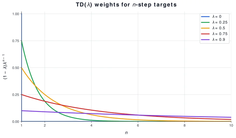
The plot shows this weight as a function of $n$. In the algorithm, $n$ is an integer, but the smooth curves make the geometric decay easier to see.

In finite episodic tasks, $\lambda = 1$ is handled as the limiting case where the return becomes the full Monte Carlo return. We will not need the full TD($\lambda$) machinery for basic algorithms, but it is useful to understand the spectrum:

• Monte Carlo waits longer and uses less bootstrapping.
• One-step TD updates sooner and uses more bootstrapping.
• TD($\lambda$) sits between those extremes.

Exploration

We now have two ways to estimate $q_\pi(s, a)$ from samples: Monte Carlo returns and TD targets, but both methods depend on the samples we actually collect. If the policy never tries action $a$ in state $s$, then we do not get returns or TD targets for $(s, a)$, and we cannot estimate $q(s, a)$ well. As a consequence, the improved policy may never discover actions that would maximize the total discounted reward.

This is another consequence of being model-free. Because we do not know $p(r, s^\prime \mid s, a)$, we cannot reliably predict what an untried action would do. The data-collecting policy therefore has to try alternatives sometimes instead of always choosing the current greedy action. That is exploration.

Before writing control algorithms, we should make action selection explicit. A policy is a rule for choosing actions. It may be deterministic, like:

or stochastic, in which case we sample from an action distribution:

The stochastic policy we will use is $\epsilon$-greedy. In each state, look at the current $q(s, a)$ values and find the action that looks best. Most of the time, choose that action. With probability $\epsilon$, choose randomly so that other actions still get tried. The greedy choice exploits the current estimates. The random choice explores actions that may look worse now but could teach us something important. Balancing these two forces is the exploration-exploitation problem.

One downside of constant $\epsilon$-greedy exploration is that we keep paying an exploration cost even after we have learned a good policy. Over time, we want to maximize returns, not keep probing random actions. A common fix is to decay $\epsilon$ over training: start high to explore broadly, then lower it so the agent increasingly exploits what it has learned. That said, in non-stationary environments where the rules or rewards can change over time, keeping some exploration permanently makes sense.

Generalized Policy Iteration

We now have the ingredients for model-free control:

• An $\epsilon$-greedy policy usually chooses the action with the largest current $q(s, a)$ but still tries other actions.
• Monte Carlo and TD give us ways to estimate $q_\pi(s, a)$ from sampled rollouts.

So far, Monte Carlo and TD were only prediction tools: keep a policy fixed and estimate how good its actions are. For control, we do not need to invent a new framework. We can reuse Policy Iteration from the previous article and run the same two-step loop, now with sampled estimates:

1. Policy evaluation: estimate action-values for a target policy.
2. Policy improvement: make the policy prefer actions with larger estimated values.

The model-based version used the transition dynamics to evaluate a policy. Here we do not have those dynamics, so evaluation has to come from samples. The improvement step also changes slightly: instead of always choosing the action with the largest $q(s, a)$, the policy keeps some random exploration so that training continues to produce useful data.

This is Generalized Policy Iteration (GPI). The two steps are still distinct, but they can be interleaved at different rates. We can evaluate for many episodes and then improve, or we can improve after every small update to $q$. The algorithms below differ mostly in what target they use for evaluation: complete returns, sampled next actions, an average over next actions, or a greedy optimality target.

Monte Carlo Control

Monte Carlo Control uses complete returns for the evaluation part. Generate an episode with the current policy, use the observed returns to update $q(s, a)$, then refresh the policy from the new estimates: in each state, the action with the largest $q(s, a)$ becomes the greedy choice, while random exploration with probability $\epsilon$ remains.

A basic version is:

1. Generate an episode using the current policy $\pi$.
2. For each visited pair $(S_t, A_t)$, compute the return $G_t$ from that point in the episode.
3. Update the running average for $q(S_t, A_t)$.
4. After the $q$ update, recompute the greedy action in each state, while keeping probability $\epsilon$ for random exploration.
5. Repeat.

SARSA

SARSA keeps the same policy-evaluation, policy-improvement loop, but replaces the complete Monte Carlo return with a one-step TD target.

For the one-step target, we need to know which action the policy will take in the next state. So the sampled piece is:

This is where the name SARSA comes from: state, action, reward, state, action. If the sampled step is $(s, a, r, s^\prime, a^\prime)$, the target is:

and the update becomes:

If $s^\prime$ is terminal, there is no next action and no future value, so the target is just:

A simple SARSA loop is:

1. Choose $a \sim \pi(\cdot \mid s)$, take it, and observe $r$ and $s^\prime$.
2. If $s^\prime$ is not terminal, choose $a^\prime \sim \pi(\cdot \mid s^\prime)$ using the same policy.
3. Update $q(s, a)$ toward $r + \gamma q(s^\prime, a^\prime)$, or toward $r$ if $s^\prime$ is terminal.
4. After the $q$ update, recompute the greedy action in each state, while keeping probability $\epsilon$ for random exploration.
5. If the episode is not done, set $s \leftarrow s^\prime$, $a \leftarrow a^\prime$, and continue.

The important detail is that $a^\prime$ is not arbitrary. The Bellman expectation equation for $q_\pi$ says that after reaching $s^\prime$, we continue with policy $\pi$. If we approximate that next-action expectation with one sampled action, then the sampled action has to come from $\pi(\cdot \mid s^\prime)$. This is the core reason SARSA is on-policy: the policy being evaluated must also generate the next sampled action. If $\pi$ is $\epsilon$-greedy, then the target includes that exploration, so SARSA learns the value of the policy it actually follows. We will talk more about off-policy vs. on-policy in the next section.

Expected SARSA

Expected SARSA uses the alternative we mentioned in the TD section. SARSA samples one next action and uses:

Expected SARSA keeps the action expectation instead. After observing $(s, a, r, s^\prime)$, it averages over the actions that policy $\pi$ could take in $s^\prime$:

The update is:

For a terminal next state, the target is again:

The difference is small but useful. SARSA asks which next action the policy happened to sample. Expected SARSA asks for the average value under all actions the policy might sample. The cost is that we have to know the action probabilities $\pi(a^\prime \mid s^\prime)$ and sum over the available actions, which is cheap when the action set is small and discrete.

A simple control loop is:

1. Choose $a \sim \pi(\cdot \mid s)$, take it, and observe $r$ and $s^\prime$.
2. Update $q(s, a)$ toward $r + \gamma \sum_{a^\prime} \pi(a^\prime \mid s^\prime) q(s^\prime, a^\prime)$, or toward $r$ if $s^\prime$ is terminal.
3. After the $q$ update, recompute the greedy action in each state, while keeping probability $\epsilon$ for random exploration.
4. Continue from $s^\prime$.

Unlike SARSA, this update does not need to carry a sampled $a^\prime$ forward. The sampled tuple is really $(s, a, r, s^\prime)$. The final “A” in Expected SARSA is the action distribution inside the expectation, not a sampled action in the update.

On-policy vs. Off-policy

Once the behavior policy includes exploration, we need to separate two ideas:

• The behavior policy is the policy that collects data.
• The target policy is the policy being learned or evaluated.

In on-policy learning, the behavior policy and target policy are the same. The update evaluates the policy that actually acts.

In off-policy learning, they can be different. It is like watching over someone else’s shoulder while they play a game: their actions generate experience, but we can use that experience to learn about a different way of playing. Watching strong players is especially useful because their trajectories spend more time near good decisions, so the behavior policy does not have to explore as much.

The Bellman expectation equation makes the target policy explicit. It evaluates $q_\pi$, the value of taking one action and then following policy $\pi$:

After we replace the outer sum with a sampled transition, the model-free update no longer needs explicit transition probabilities. It only needs an observed $(s, a, r, s^\prime)$. That transition may have been collected by the current policy, by another behavior policy, or from an existing dataset. Once action $a$ was taken in state $s$, the observed $r$ and $s^\prime$ are samples from the environment dynamics $p(r, s^\prime \mid s, a)$.

The target policy $\pi$ appears in a different place: the next-state action distribution. That is the inner sum:

So the key question is not only “who collected this transition?” It is also “which policy is used inside the target?”

SARSA samples the inner expectation with one actual next action $a^\prime$. If we are evaluating $\pi$, that sampled $a^\prime$ must come from $\pi$. In the basic control algorithm, the same $\epsilon$-greedy policy both acts and appears in the target, so SARSA is on-policy.

Expected SARSA does not sample $a^\prime$. It computes the inner expectation directly from the target policy’s action probabilities. That gives two valid cases:

• On-policy Expected SARSA: the behavior policy and target policy are the same, so transitions come from $\pi$ and the expectation is also under $\pi$.
• Off-policy Expected SARSA: a behavior policy collects $(s, a, r, s^\prime)$, but the expectation is computed under a different target policy $\pi$.

Plain Monte Carlo Control is also on-policy, but over a longer horizon. Its target is the full return:

This return is not just about the first action. It also depends on the later actions in the episode. If those later actions were chosen by the current policy $\pi$, then $G_t$ is a sample of $q_\pi(S_t, A_t)$. So plain Monte Carlo Control is on-policy because the episode is generated by the same policy whose action-values the return is estimating. The policy may still improve between episodes; on-policy does not mean the policy is frozen forever.

Q-learning is different again: it does not use the Bellman expectation equation for a fixed policy. It uses the Bellman optimality equation, whose next-state target is greedy. The behavior policy can explore, but the update target is the value of acting greedily after the sampled transition.

Q-learning

Q-learning takes the Value Iteration idea and applies it to action-values. Instead of evaluating a fixed policy with the Bellman expectation equation, it uses the Bellman optimality equation for $q^*$. The question is: if we take action $a$ in state $s$, and then act optimally, what return do we expect?

There is no policy distribution in this equation. The maximum already encodes the idea that, from the next state onward, the agent chooses the best available action. Once we know $q^*$, an optimal policy falls out by acting greedily:

The Bellman optimality equation still contains transition probabilities, so computing the right-hand side exactly requires a model of the environment. Q-learning is the model-free, sampled version of that idea. One observed transition:

replaces the expectation over all possible outcomes. The sampled optimality target is:

The update is:

The maximum is computed from the current table of action-values. In the next state $s^\prime$, look at every available action $a^\prime$ and take the largest current estimate:

This does not mean the agent must actually take that action next. The maximum is only used to compute the update target. The next real action is still chosen by the behavior policy. In fact, the agent does not even need to be acting now: the transitions could come from a logged dataset of past behavior.

Q-learning is off-policy for two connected reasons:

• The Bellman optimality equation does not require an explicit policy. The target is greedy because of the maximum.
• The sampled transition $(s, a, r, s^\prime)$ is only used to estimate the environment dynamics. It can come from any behavior policy, including an existing record of actions, as long as the data covers enough state-action pairs.

A simple Q-learning loop is:

1. Choose $a$ in state $s$ using the behavior policy. For example, use $\epsilon$-greedy with respect to the current $q$ values.
2. Take $a$, observe $r$ and $s^\prime$.
3. Update $q(s, a)$ toward $r + \gamma \max_{a^\prime} q(s^\prime, a^\prime)$, or toward $r$ if $s^\prime$ is terminal.
4. After the $q$ update, recompute which actions the behavior policy treats as greedy.
5. If the episode is not done, set $s \leftarrow s^\prime$ and continue.

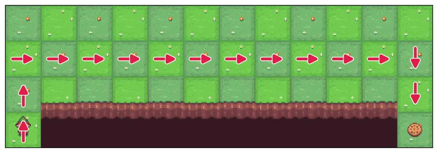
Cliff Walking Example

Let’s ground the algorithms in another small grid-world game. Each cell is a state $s$, and from each non-terminal state the agent can move up, down, left, or right.

The agent starts in the bottom-left cell and has to reach the goal in the bottom-right cell. The dark cells between them are the cliff. Every normal step gives reward $-1$. Stepping into the cliff gives reward $-100$ and sends the agent back to the start. Reaching the goal ends the episode.

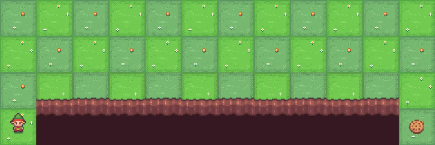
This environment is useful because two routes are both reasonable, depending on what policy we are evaluating. The shortest route goes directly above the cliff. It reaches the goal quickly, but one exploratory move downward can be very expensive. A safer route goes one row higher. It takes a few extra steps, but it gives the behavior policy more room for mistakes: even if exploration makes the agent choose a random action, it is less likely to step straight into the cliff and receive the $-100$ penalty.

The images below show the deterministic greedy policy extracted after training. They do not show the random exploratory moves taken during training. They show what each learned $q$ table would do if we acted greedily afterward.

That detail matters. For Monte Carlo Control, SARSA, and Expected SARSA, the $q$ values were learned for an $\epsilon$-greedy policy. The final plot removes exploration by taking the best action in each state, but the values behind those arrows still include the cost of possible future exploratory moves. So the greedy path in the image does not have to be the shortest deterministic path.

Monte Carlo Control

Monte Carlo Control does find a route to the goal, but the greedy route in this plot is less direct.

The main reason is that Monte Carlo Control updates from the full return of the episode. In Cliff Walking, falling into the cliff gives $-100$ and sends the agent back to the start, but it does not end the episode. So if an exploratory move hits the cliff later in the episode, that penalty and the recovery steps become part of the return for earlier state-action pairs too. With $\epsilon$-greedy episodes, those full returns can be noisy, and the learned action-values may make a safer-looking route appear best.

This does not mean Monte Carlo is implemented incorrectly. It means that, in this environment and with this exploration setup, full-episode returns have high variance. The bootstrapping methods below use shorter targets, so they usually stabilize the path faster.

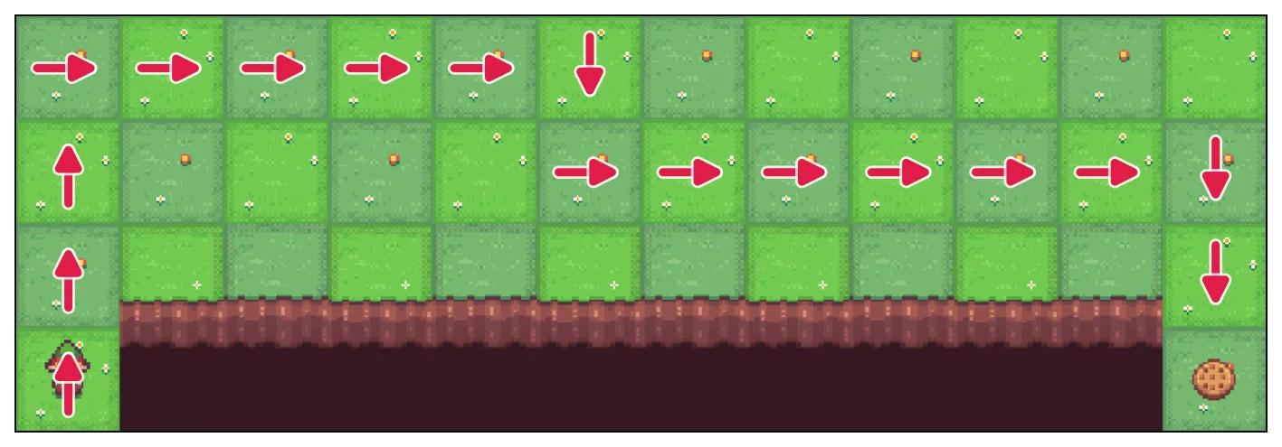
SARSA

SARSA learns the most cautious route in this run: it goes to the top row first, then moves right. This matches the usual cliff-walking effect described by Sutton and Barto: SARSA is on-policy, so it learns action-values for the $\epsilon$-greedy policy that is actually used during training. Most of the time the agent follows the current best action, but with probability $\epsilon$ it takes a random action. Near the cliff, a random move down can cost $-100$.

After reaching $s^\prime$, SARSA chooses the next action $a^\prime$ with the same $\epsilon$-greedy policy and uses that action in the update:

Imagine the agent is on the middle path and moves to a state $s^\prime$ closer to the cliff. From there, $\epsilon$-greedy can still sample the dangerous action down. After enough falls, $q(s^\prime,\text{down})$ becomes very low because that action leads to the $-100$ cliff penalty. If down is the sampled $a^\prime$, SARSA uses this low action-value in the target for the previous move. In other words, the low $q(s^\prime,a^\prime)$ helps update $q(s,a)$ for the middle-path move. So the middle-path move can look bad too.

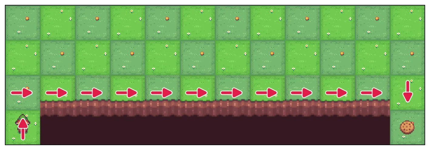
Expected SARSA

Expected SARSA learns the middle route. It is still on-policy in this setup, so it is also evaluating the $\epsilon$-greedy policy that may explore. The difference is that it does not wait to see which single $a^\prime$ was sampled. After reaching $s^\prime$, it asks what would happen on average if the agent followed the $\epsilon$-greedy policy from there:

If $s^\prime$ is close to the cliff, that average includes the small chance that exploration picks down and falls. So Expected SARSA already knows that states near the cliff are risky under the $\epsilon$-greedy policy. But it also sees that going all the way to the top row costs extra steps. In this run, the middle route has the best balance: safer than the cliff edge, but shorter than the top path.

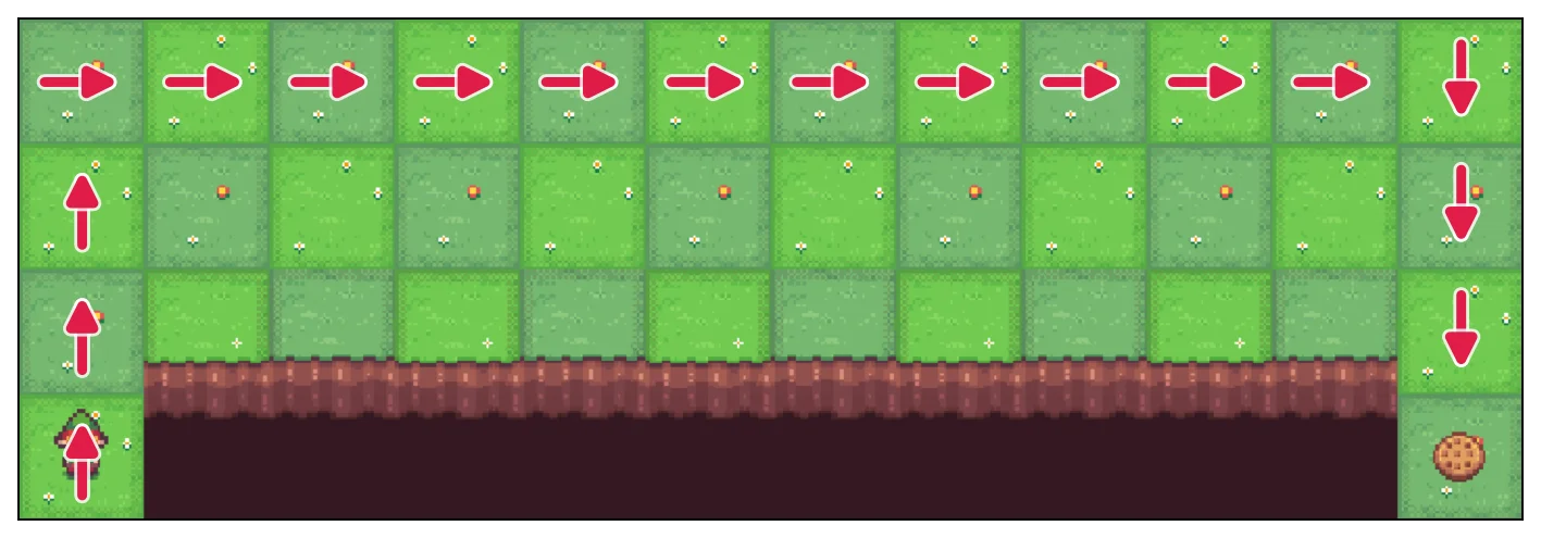
Q-learning

Q-learning learns the shortest route just above the cliff. It is off-policy: the behavior policy may still be $\epsilon$-greedy during training, but the update learns action-values for a greedy target policy. Its target uses the best next action:

So after a move reaches $s^\prime$, Q-learning does not ask what random exploratory action might be sampled there. It assumes the agent will take the best-known action. Under that assumption, the path directly above the cliff is attractive: it reaches the goal in the fewest steps, and the greedy policy will not intentionally move down into the cliff. The agent may still fall during training because the behavior policy explores, but that exploration risk is not part of the policy Q-learning is learning.

Exercise

Want to test your understanding? I prepared an exercise for this lesson in my Reinforcement Learning Course.

Summary

The main shift in this lesson was from planning with a known model to learning from sampled interaction. When we do not know the transition probabilities, learning only $v(s)$ is not enough for control, because we cannot look ahead through the model to compare actions. Instead we learn $q(s, a)$, which lets us choose actions directly:

We also saw two broad ways to estimate action-values from data. Monte Carlo methods wait until an episode ends and use the complete return. Temporal Difference methods update after each step by bootstrapping from the estimates they already have. SARSA, Expected SARSA, and Q-learning are all TD control methods, but their targets differ: a sampled next action, an expected next action, or a greedy maximum. The cliff-walking example made that difference visible, since these targets lead to different preferred routes.

Because the agent only learns from actions it actually tries, exploration is not optional. An $\epsilon$-greedy behavior policy keeps collecting useful samples while still exploiting what has already been learned.

Finally, we separated on-policy from off-policy learning. SARSA learns about the same policy it uses to act. Expected SARSA can be either on-policy or off-policy, depending on whether its expectation uses the behavior policy or a separate target policy. Q-learning is off-policy because it can explore during training while learning the greedy policy.

Towards Deep Q-learning

So far $q(s, a)$ was treated as a table. That is enough for small environments, but it will not scale to images, continuous state vectors, or very large state spaces. Neural networks can address this scaling problem by approximating action-values with parameters $\theta$:

Once we do that, the algorithm needs extra machinery. Neural networks are sensitive to correlated data, and Q-learning targets move as the network changes. This is where experience replay and target networks become important. We will cover those ideas in the next article when we move from tabular Q-learning to Approximate methods.