Reinforcement Learning 104: Deep Q-Networks

Introduction

In the previous article, we replaced the tabular action-value function $q(s, a)$ with a parameterized approximation: $q_\theta(s, a)$. We will use neural networks to approximate $q_\theta(s, a)$.

Deep Q-Network (DQN) is the version of approximate Q-learning that made it practical at a scale. When we combine Q-learning with neural networks, then we must deal with the instability created by correlated data, moving targets, changing behavior distributions, and large TD errors. This article presents solutions to deal with those problems.

Before we continue, we need to understand why we moved forward with approximate Q-learning, not approximate SARSA or Expected SARSA.

Why not SARSA?

SARSA is an on-policy algorithm: it learns the value of the policy that is currently acting. Its target uses the actual next action $a^\prime$:

The important detail is $a^\prime$. For SARSA to be truly on-policy, this action should come from the current policy. If we keep a history of old transitions and train on one of them later, the policy may have already changed, so the stored $a^\prime$ is stale.

Q-learning avoids this issue because it is off-policy. The behavior policy can explore and collect transitions, while the update still trains toward the greedy policy:

This fits neural-network training better because the same old transition can be reused many times, and each reuse can produce another gradient update to the weights.

Expected SARSA can also be off-policy. Its target is:

Expected SARSA with an $\epsilon$-greedy policy learns values under the assumption that the agent will keep exploring in the future. In other words, the learned $q_\theta(s,a)$ estimates the return of a policy that sometimes deliberately takes non-greedy actions.

That is not what we want because usually we want to play the best policy we found, not continue making random exploratory moves. If we are playing for the championship, we care about winning the game, not about gathering more data.

One caveat is that this does not mean on-policy methods are worse by default. Later, when we discuss A3C, we will see another way to make fresh on-policy data more efficient.

Now, let’s go back to DQN and problems we outlined in the previous article.

Problem 1: Correlated Data

Stochastic gradient descent works best when batches give a useful estimate of the training objective. In supervised learning, we sample examples independently from the same training distribution and use the minibatch gradient as an unbiased estimate of the expected gradient:

Consecutive RL samples are not like independently sampled training examples. During one episode, adjacent states are strongly correlated.

Imagine an agent watching the ball move across the screen. Frame $t$ and frame $t+1$ are almost the same. If we train directly on the latest transition at every step, the network sees a long stream from one small region of experience. The gradient points too strongly toward what just happened and too weakly toward the broader game.

There is also a distribution problem. In supervised learning, the dataset is usually fixed. In RL, the behavior policy creates the data. If $q_\theta$ changes, then an $\epsilon$-greedy policy may choose different actions and reach different states. If we train only on the newest transitions, the training distribution can immediately become dominated by whatever the current policy just visited, instead of staying stable and well mixed.

Experience Replay

DQN appends each transition to a replay buffer $\mathcal{D}$ and trains on random batches $B$ sampled from it. This helps in several ways.

1. It breaks short-term correlations. A random batch may contain transitions from different episodes, different game situations, and different moments in training. The samples are not truly independent, but they are much less correlated than consecutive frames.

2. It improves data efficiency. One transition can be used in many gradient updates of our neural network. This matters because environment interaction is often the expensive part.

3. It slows sudden shifts in what the network trains on. This makes learning more stable: a small change in the current policy does not immediately replace the whole training batch with new, similar transitions.

Other way to think about replay batch is that it can be viewed as a sample-based model of the world. A real model would estimate:

and let us ask what would happen for arbitrary state-action pairs. A replay buffer does not do that. It cannot generate new transitions for states and actions we never tried, but it is a non-parametric collection of one-step samples from the environment.

What are disadvantages of replay?

1. If a replay buffer is large, then it is memory intensive. For Atari, one uint8 grayscale frame is $84 \times 84 = 7{,}056$ bytes. A transition contains $s_t$ and $s_{t+1}$, each a stack of 4 frames, so naive storage needs $8 \times 7{,}056 = 56{,}448$ bytes per transition i.e. ~56GB for $1M$ transitions. Practical buffers avoid most of this duplication by storing frames once and reconstructing overlapping states, which is why Atari replay buffers are often closer to ~7GB.

2. Uniform random sampling to form a batch is not optimal as it treats all transitions as equally useful. In reality, some transitions have larger TD errors or contain rare rewards. Prioritized replay improves this idea by sampling more informative transitions more often, but vanilla DQN uses uniform sampling.

3. Replay trains on transitions collected by older versions of the policy. Q-learning can use them because it is off-policy, but too much old experience can slow adaptation when the current policy starts reaching different states. Having said that, bigger replay buffer is not always better.

Problem 2: Moving Targets

Experience replay helps with correlated data, but it does not solve the moving target problem. In approximate Q-learning, the target is:

In the previous article, we established that we use semi-gradients for targets $y(\theta)$, so during one gradient update the target is treated as fixed. However, this is not enough. Once we update the network parameters $\theta$, the target $y(\theta)$ also changes, because the same network is used both to predict $q_\theta(s,a)$ and to build the bootstrap target $y(\theta)$.

Why is this a problem? Is it because the target is wrong? No. Bootstrap targets are usually wrong. That is expected. For example, consider the scalar recursive equation:

The true solution is:

Suppose we start from $q_0 = 0$. It does not matter that $q_0$ is wrong. If we keep applying the update:

we get:

Every intermediate value is wrong, but the sequence still moves toward the fixed point. That is the core idea behind the Bellman optimality equation, contraction mappings, and the Banach fixed-point theorem. The target does not need to be correct at every step, but it needs to be a useful next approximation.

The problem in DQN is different. We are not applying the exact recursive equation to the whole action-value function, but we are learning from finite, noisy samples using gradient descent. If we just use a noisy sample to update $q_k$, then training might behave in a very unpredictable way. Ideally, we would like to do something closer to this:

1. Keep an old action-value function $q_0$ fixed.
2. Use many noisy samples and many gradient updates to learn a better approximation $q_1$.
3. Once $q_1$ has been fitted reasonably well, replace $q_0$ with $q_1$.
4. Repeat the process.

In other words, we do not want the target to change every time the online network takes a single gradient step. We want to hold the previous approximation fixed for a while, train the new approximation against it, and only then move to the next step of the recursive process. It is then more similar to how recursive Bellman optimality equations work.

Target Network

To apply this idea in practice, DQN introduces a second neural network called the target network, with parameters $\theta^-$. DQN separates the network being trained from the network used to build the bootstrap target.

There are two networks:

• The online network $q_\theta$, updated by gradient descent.
• The target network $q_{\theta^-}$, used to compute bootstrap targets.

The target becomes:

The online network is still trained with batches $B$ sampled from a replay buffer.

During these gradient updates, the target network parameters $\theta^-$ are held fixed. This means the online network is repeatedly trained against targets generated by the same fixed action-value approximation. Then periodically, the online network copies its parameters to the target network:

Conceptually, the target network plays the role of the old approximation $q_0$. The online network tries to learn a better approximation $q_1$ using many noisy samples and gradient updates. After some time, $q_1$ becomes the new fixed reference point, and the process continues. This makes training less reactive to noisy samples and closer in spirit to approximate value iteration, although there are still no convergence guarantees like in the tabular setting.

Problem 3: Unstable Gradients

The TD error for one transition is:

For squared loss, the gradient has the form:

So the size of the TD error directly scales the update. Since action-values estimate discounted sums of rewards, larger reward scales lead to larger target values and larger TD errors. If rewards have very different magnitudes across environments, then the same learning rate can be too small for one environment and too large for another.

Reward Clipping

DQN clips rewards to:

It makes true optimal Q-values bounded by roughly:

For $\gamma = 0.99$, that is $100$. This gives good gradients in a pragmatic sense: the TD errors are kept in a range where one learning rate can work across many games. Without clipping, the scale can be much larger and very different across games.

Reward clipping has also a cost. If one action gives reward $+1$ and another gives reward $+100$, clipping makes both immediate rewards equal to $+1$. The agent can no longer distinguish good rewards from great rewards at that time step. It learns from signs and frequencies more than from exact reward magnitudes. So reward clipping is more like an engineering trick to make learning process stable.

Vanilla DQN

Now we can combine all these ideas and implement a basic DQN training algorithm.

1. Initialize the online network $q_\theta$.
2. Initialize the target network with the same parameters: $\theta^- \leftarrow \theta$.
3. Initialize a replay buffer $\mathcal{D}$.
4. Act with an $\epsilon$-greedy behavior policy based on $q_\theta$.
5. Store each transition $(S_t, A_t, R_t, S_{t+1})$ in $\mathcal{D}$.
6. Sample a batch from $\mathcal{D}$.
7. For each sampled transition, compute:

8. Update $\theta$ by minimizing loss function:

9. Periodically update the target network with a hard copy of the online network.

This is vanilla DQN: approximate Q-learning with replay buffer, a target network, and reward clipping.

Atari Pong Demo

Pong is a two-player Atari game. Here, vanilla DQN uses a Convolutional Neural Network that sees the state as the last four frames stacked together. After about 10 hours of training on a MacBook, the learned policy controls the paddle on the right and starts exploiting certain strategies that might feel like reward hacking.

Implementation

Feel free to take a look at my implementation on GitHub. I recommend implementing it yourself rather than having an agent do it. It is the best way to learn.

Tips & Tricks

There are a few practical issues that can show up when training vanilla DQN on Atari games.

1. Store frames as uint8 in the replay buffer to save memory, then convert and normalize them on the GPU:

states = states.to(self.device).float().div_(255.0)

2. If learning stalls early, check the gradient norms. In my runs, very small gradients with Adam made the model fail to learn. Using a larger Adam epsilon helped:

self.optimizer = Adam(self.policy_network.parameters(), lr=config.learning_rate, eps=1e-4)

3. I also used LeakyReLU instead of ReLU in the convolutional neural network to avoid dying ReLU neurons.

nn.LeakyReLU(negative_slope=0.01)

4. Atari environments return both terminated and truncated. Only true terminations should stop bootstrapping; time-limit truncations can still use the next-state Q-value.

transition = Transition(state=state, action=action, reward=clipped_reward, next_state=next_state, done=terminated)

Prioritized Replay Buffer

Uniform replay treats every stored transition as equally useful. That is simple and it already helps a lot, but it is not how learning usually feels. Some transitions are boring because the network already predicts them well. Others are surprising: the reward was unexpected, the state was rare, or the bootstrap target disagrees strongly with the current estimate. The TD error gives us a simple way to measure that surprise:

If $|\delta_i|$ is large, then transition $i$ currently creates a large learning signal. Prioritized replay uses this idea by sampling those transitions more often than transitions with small TD errors. A common priority is:

where $\epsilon > 0$ keeps every transition sampleable. Without this small constant, a transition with zero priority might never be seen again, even though it could become useful later after the network changes. Then the sampling probability is:

The parameter $\alpha$ controls how much prioritization we use. If $\alpha = 0$, then $p_i^\alpha = 1$ for every transition, so we end up with uniform replay. If $\alpha$ is larger, high-error transitions are sampled more often. In practice, a common choice is $\alpha = 0.6$. It is enough to prefer high-error transitions, but not so aggressive that the replay buffer is dominated only by the largest errors.

So we changed our sampling distribution. How does that affect the gradient? Before, in uniform replay, we sampled uniformly from the $N$ stored transitions:

With uniform replay, the expected minibatch gradient estimates the average gradient over the whole buffer:

Prioritized replay samples transition $i$ with probability $P(i)$ instead, so before correction the expectation becomes:

That is the bias introduced by prioritized sampling. High-priority transitions are no longer just seen more often, but they also count more in expectation. To correct that bias, multiply each sampled gradient by the ratio between its uniform probability and its prioritized probability:

Then the weighted prioritized gradient becomes the uniform replay gradient again:

This may look like it removes the benefit of prioritized replay, but it does not. The bias correction changes the weight of a transition after it has already been sampled. It does not make the sampling process uniform again. High-priority transitions are still selected more often, so the agent spends more updates looking at them.

Implementation-wise, we still need a way to sample high-priority transitions efficiently. More on that later, but once we have these high-priority samples in the batch, we correct the bias by weighting their losses. For the full correction, the weight is:

In PyTorch, this just means computing a per-sample loss for each sampled transition $i_k$, multiplying it by its weight, and then averaging over the batch:

In practice, Prioritized Replay Buffer often does not use the full correction immediately. It introduces a parameter $\beta$:

Here $N$ is the number of transitions in the replay buffer. The parameter $\beta$ controls how strongly we correct the sampling bias. If $\beta = 0$, there is no bias correction. If $\beta = 1$, the bias correction is full.

Sometimes we intentionally want stronger gradients from high-priority samples. Early in training, the policy, targets, and priorities are changing quickly, and high-error transitions often contain the useful signal the network is currently missing. If we fully correct the bias immediately, many of those transitions are downweighted after we sampled them. That can make prioritization less aggressive exactly when we want it to move learning quickly.

So Prioritized Replay Buffer usually starts with weaker correction, for example $\beta = 0.4$, and anneals $\beta$ upward toward $1.0$ during training. Later, as the value estimates become more stable, stronger correction reduces the extra influence of high-priority samples and makes the update less biased relative to uniform replay.

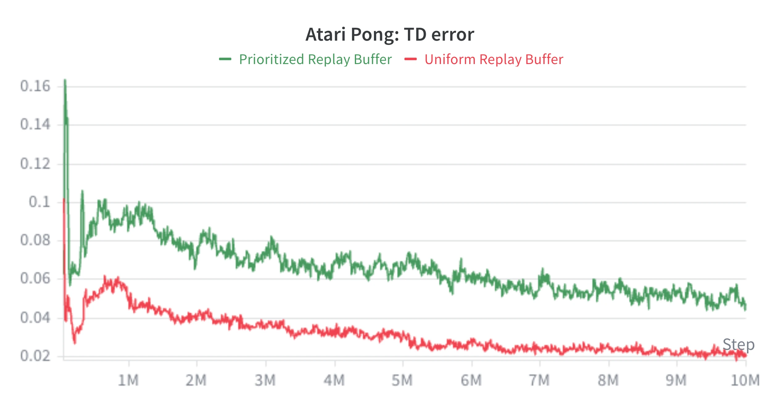
Training Curves

Here is one Pong run comparing uniform replay with prioritized replay. The prioritized replay agent reaches positive returns earlier, although both runs end up close after enough environment steps.

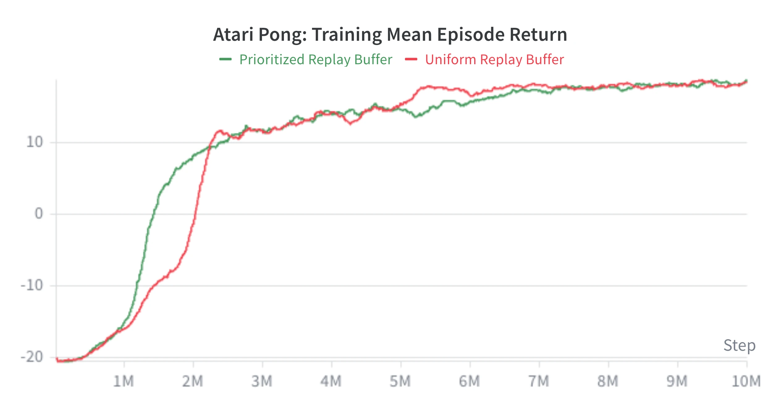
Since high-priority transitions appear more often in batches, the sampled batch TD error can stay higher while the policy improves.

Implementation

The replay buffer itself can still be a normal circular buffer: arrays for states, actions, rewards, next states, and done flags. The extra part is one priority per stored transition. The algorithm is straightforward:

1. Sample a batch from the replay buffer using priorities to form a probability distribution.
2. Train on that batch and compute the TD error for each sampled transition.
3. Convert each TD error into a new priority.
4. Store that priority next to the transition in the regular replay buffer.

New transitions do not have a TD error yet, so they usually get the current maximum priority. That makes sure they can be sampled at least once.

The naive sampling approach is to build a probability distribution over the current buffer from these priorities, then sample from that distribution. This works, but it requires to scan a whole replay buffer with time complexity $O(N)$.

A sum tree is a data structure that makes this weighted sampling efficient. It stores priority sums in a binary tree, so we can sample a transition in $O(\log N)$ instead of scanning the whole buffer. Adding a new transition or updating an existing priority is also $O(\log N)$. The actual transitions do not live in the tree, they still live in a replay buffer. The tree plays a role of an indexing data structure and maps priority mass to replay-buffer indices.

For the implementation details, see my prioritized replay buffer code.

Overestimation Bias

Target networks made the bootstrap target change more slowly, so we could apply recursive Bellman optimality equations with more confidence and less noise. I also mentioned that target estimates were always wrong, but it was fine, because that was the nature of Bellman updates.

Though, you can also imagine that if targets were perfectly correct, then the algorithm would converge much faster. Let’s first understand what is wrong with our target estimate. For one sampled non-terminal transition, the ideal target for that sample would be:

DQN does not know $q^*$ so it trains on the estimate:

During that gradient update, $\hat y$ is just a fixed number. Below is a mathematical analysis of fixed target-network action-value estimates being noisy estimates of the true action-values.

For each next action $a^\prime$, write the target-network estimate as the true action-value plus an estimation error $\epsilon_{a^\prime}$.

Then each next action-value estimate is correct on average:

Based on that, if we averaged out the noise before taking the max, the max term would match the true optimal value of the sampled next state:

That is the reference we would want the $max$ term to match. If the max term were equal to this quantity, then the target estimate $\hat y$ would be an unbiased estimator of $y^*$:

Unfortunately, the actual DQN target maximizes the noisy estimates before averaging, so $\mathbb{E}_\epsilon[\hat y] \neq y^*$. It means that the target estimate $\hat y$ is a biased estimator of $y^*$.

We don’t achieve the desirable unbiased estimator, because the estimate from DQN is larger. That’s why we call it overestimation bias.

This follows from Jensen’s inequality, because the max over actions is a convex function of the action-value vector.

For a tiny example, assume two actions have true value $0$, and each estimate is independently either $-1$ or $+1$ with equal probability. Each row below has probability $\frac{1}{4}$.

If we average before the max, there is no overestimation:

If we take the max before averaging, there is:

A takeaway is that DQN can learn values that are too high, not because the rewards or true next-state values are high, but because the bootstrap target repeatedly selects action estimates with positive error terms $\epsilon_{a^\prime}$.

Double DQN

In the overestimation section, the bad term was:

Double DQN changes this by not using target network to choose the action $a^\prime$ whose value will appear in the target and start using online network instead.

The online network $q_\theta$ chooses the next action:

The target network $q_{\theta^-}$ evaluates that selected action:

So the max is still there, but it is only used to choose an action index:

As you can see, the target-network value used to evaluate the selected action is not the maximum anymore, but the value at the index selected by the online network. Having said that, if we condition on the action selected by the online network, then maximization bias disappears:

You might say that the online network can be noisy too. You are right. In the expectation above we assumed that a decision $a_\theta$ was already made and we computed expectation with respect to $\epsilon^-$.

Let’s go back to the tiny two-action example from the previous section where $q^*(a_1)=q^*(a_2)=0$. Now let $\epsilon^\theta_i$ be the online-network error for action $a_i$, and let $\epsilon^-_i$ be the target-network error.

Then the online network selects one of the two actions:

The target network evaluates that selected action:

Now let’s average the Double DQN value. The selected action $a_\theta$ is determined by the online-network errors $\epsilon^\theta_1$ and $\epsilon^\theta_2$.

This equation tells us that if the noise $\epsilon^\theta$ used to select the action is independent of the noise $\epsilon^-$ used to evaluate that action, then the target network does not add a positive error on average.

In practice the two networks are not fully independent, because $\theta^-$ is periodically copied from $\theta$. Having said that, Double DQN reduces this overestimation bias rather than removing it completely.

Dueling DQN

A normal DQN directly predicts one value per action:

However in many situations, knowing that the state is good or bad is easier than knowing the exact best action. Imagine playing Pong when the ball is on the opposite side of the screen. Moving the paddle up, down, or doing nothing for one frame may lead to almost the same long-term outcome, because one slightly bad move does not decide the point. Having said that, you could say that all $q_\theta(s, a)$ share the same $v_\theta(s)$ value.

Indeed, a neural network shares hidden layers across actions, so the action outputs are not completely independent. However, to estimate $q_\theta(s, a)$ well for each action, the network has to learn what happens when those actions are taken in states where it doesn’t matter. This is a bit wasteful, and it is often better to first estimate $v_\theta(s)$ and then only use an action-specific term for the difference between actions. Dueling DQN explicitly decomposes action-values by representing them with two terms:

• A state-value term $v_\theta(s)$, which outputs one number.
• An advantage term $z_\theta(s, a)$, which outputs one number per action.

The naive decomposition is:

We train together $v_\theta(s)$ and $z_\theta(s, a)$ in a single network, but we use separate neural network outputs. After obtaining separate outputs, we compose them together to get $q_\theta(s, a)$.

The difference is:

• In the Dueling DQN, every sampled transition updates the value term $v_\theta(s)$, because $v_\theta(s)$ contributes to every action-value built from that state.

• In a normal DQN update, the TD loss is applied to the output for the sampled action $a$. The shared hidden layers can still change, but the other action outputs do not receive their own direct TD error in that update.

In other words, the network does not need to relearn the same state-quality signal separately for each action output. It can spend more capacity on estimating the state value well, and then let the advantage term learn the smaller differences between actions. This matters for temporal-difference learning, because the bootstrap target depends on having accurate next-state values. It also explains why the dueling architecture becomes more useful when the action space is large.

Now let’s look closer at the naive decomposition of $q_\theta(s, a)$:

For any constant $c(s)$:

This means that the same $q_\theta(s, a)$ can be represented in infinitely many ways. For example, the network could add $10$ to the value term and subtract $10$ from every raw score output, and the final $q_\theta(s, a)$ would not change.

At first this may look harmless, because the TD loss only cares about the final $q_\theta(s, a)$. The problem is that the two heads are supposed to give the network a useful division of work: $v_\theta(s)$ should carry the common state-quality signal, while $z_\theta(s, a)$ should carry the action-specific differences. Without a constraint, the training loss gives no reason to prefer one offset over another, so the value term and advantage term can drift together by arbitrary state-dependent constants. In that case neither has a stable meaning, and the network can waste capacity coordinating cancelling offsets instead of learning. So the decomposition needs an anchor.

One possible anchor is to subtract the largest raw advantage score:

This makes the best raw score equal to zero after normalization. It matches the intuition that if $v_\theta(s)$ means the value of the best action, then the normalized score can be interpreted as a lost opportunity: every worse action has non-positive advantage.

For example, suppose a state has two true optimal action-values:

If $v^*(s)$ is interpreted as the best action-value, then $v^*(s) = \max_a q^*(s, a) = 100$. The optimal advantage relative to that best action is:

Taking $a_2$ is therefore a $99$ point lost opportunity compared with the best available action.

In practice, Dueling DQN usually uses a mean-subtraction anchor instead:

Now the normalized scores have average zero:

So the average action-value in a state is exactly the value term:

The mean version no longer makes $v_\theta(s)$ equal to the best action-value, but it makes $v_\theta(s)$ equal to the average action-value under the network’s current outputs. That is also okay because the point of the dueling architecture is not to recover a separately supervised “true” value term and “true” advantage term. The point is to remove the arbitrary offset and give the network a stable way to build $q_\theta(s, a)$.

In practice we often use mean subtraction because it gives a smoother, more stable parameterization: the anchor depends on all action scores instead of only the maximal one. In code it is a simple change in the forward pass and neural network architecture.

def forward(self, states: Tensor) -> Tensor:
    features = self._model(states)
    value = self._value_head(features)
    advantage = self._advantage_head(features)
    return value + advantage - advantage.mean(dim=1, keepdim=True)

Final Thoughts

Vanilla DQN showed how to learn efficiently from a buffer of stored transitions instead of training only on the latest environment step. Experience replay makes the data more reusable and less correlated, while the target network makes the bootstrap target less reactive.

Prioritized replay then improves the buffer by sampling more informative transitions more often. Double DQN improves the target by reducing overestimation bias. Dueling DQN improves the network architecture by separating the shared state-quality signal from action-specific differences.

There are many more DQN improvements in the literature beyond the ones covered in this article. Rainbow and Beyond The Rainbow are useful next papers because they show how several compatible improvements can be combined into one stronger agent.

References

1. Q-learning
2. Playing Atari with Deep Reinforcement Learning
3. Human-level control through deep reinforcement learning
4. Prioritized Experience Replay
5. Deep Reinforcement Learning with Double Q-learning
6. Dueling Network Architectures for Deep Reinforcement Learning
7. Rainbow: Combining Improvements in Deep Reinforcement Learning
8. Beyond The Rainbow: High Performance Deep Reinforcement Learning On A Desktop PC